
We all know cyber threats are growing fast. That’s why we need better tools to keep our networks safe. Our project uses AI. it’s like teaching a computer to spot when something’s not right and to take action before any harm is done. Ethics are at the heart of our work. We’re making sure our AI system is fair and protects people’s privacy. We’re teaching it to make decisions the right way, without any hidden biases. Here’s how we’re doing it:
our AI learns what normal network activity looks like. When it sees something strange, it checks if it’s a real threat or just a harmless blip. This way, we don’t get alarms for no reason. Some might worry that using AI could make things more risky. But we’ve thought about that. We’re making our AI tough against attacks. It’s trained to know the difference between normal issues and serious cyber attacks, which helps it to stop false alarms.
In the fast-moving world of cybersecurity, we must stay ahead of threats. AI helps us do this by giving us smarter and quicker ways to handle security issues. Ethical hackers and security experts need to understand how to use AI tools to protect our digital spaces effectively. As AI and ML evolve quickly, they bring up ethical concerns. Biases in data can cause unfair results. AI's complex algorithms can be unclear, making it hard to see how decisions are made. This can make people trust AI less, especially in important areas like healthcare and law. Using personal data without permission, or using AI to make deepfakes or plan cyberattacks, shows we need strong security rules. We need to make sure AI isn't misused and that we use it ethically. It's important to make sure people agree to use their data, and that there's clarity and responsibility in how AI decisions are made. We should keep to ethical standards and be transparent to make sure AI does good and minimizes harm.
Our study is about network security, looking at firewalls, and IDS/IPS that protect networks from unauthorized access and threats. AI integration is revolutionizing security, leading to safer digital interactions. Our research consists of theoretical exploration with practical analysis, precise real-world data, and algorithms. The result is an advanced network intrusion detection system proficient in spotting anomalies and preempting potential network attacks. This process includes machine learning and pattern recognition to gain insights from historical security data and patterns. It allows us to identify irregularities and possible security risks.
AI-driven systems are also equipped with automated incident response, predictive analytics, and overall automated functions. We have real-time insights and can swiftly adapt to new attack vectors without requiring frequent rule updates and reducing false positives, which happens with the help of advanced analytics.
IAM (Identity and access management) is a set of processes and technologies used to manage users' identity and control access to IT resources within an organization.
IDS (Intrusion Detection System) is a monitoring solution for detecting cybersecurity threats to an organization. We have 2 main types: HIDS and NIDS. HIDS stands for Host intrusion detection system, and it is only used to delete potential threats and security risks on an endpoint device or a host, while NIDS stands for Network Intrusion Detection system, and it is set at the network level.
IPS ( Intrusion prevention system) is an active protection system like the IDs, it attempts to identify potential threats based on monitoring features of a protected host or network and can use signature, anomaly, or hybrid detection methods.
SIEM is a powerful tool for network anomaly detection systems using machine learning, so we explored multiple pioneering cases where I need cybersecurity.
Phishing is a type of social engineering attack that involves sending deceptive messages via email or text messages. Most of the phishing attacks take place over email messaging.
Vishing (voice phishing) such as phone calls to deceive individuals into providing sensitive information.
Smishing stands for SMS phishing, it uses text messages to trick individuals into providing sensitive information or clicking on malicious links. These messages often appear urgent, claiming issues with bank accounts, passwords, or other critical matters.
Pharming is a sophisticated type of fraudulent activity that redirects internet users to fake websites to steal personal or financial information, such as login credentials, credit card details, or social security numbers.
Whaling targets high-profile individuals within an organization, such as CEOs or top executives.
It is always best if you combine your own knowledge of manual phishing attack detection with a phishing detection tool for the best possible security.Decision Trees are a popular machine learning algorithm used for both classification and regression tasks. They are a type of supervised learning algorithm that can be used for predictive modeling. The basic idea behind a decision tree is to recursively partition the data into subsets based on the values of input features, with the goal of making predictions about the target variable.
Logistic Regression is a statistical model used for binary classification problems where the outcome variable (dependent variable) is categorical and has two classes. Despite its name, logistic regression is a classification algorithm rather than a regression algorithm.
Random Forest Classification often performs well on a variety of datasets and is less prone to overfitting compared to more complex models.
Random SearchCV processes a specified number of random in combination with parameters selected and evaluated. This method is computationally less expensive than GridSearchCV (which uses all possible combinations) and can be more efficient when dealing with a large number of hyperparameters.
We’ll delve into AI’s role in enhancing cybersecurity tools, including AI-enriched SIEM systems, AI-driven firewalls, and AI-integrated IDS/IPS, which are revolutionizing cybersecurity. AI-powered SIEM systems surpass traditional counterparts by enhancing data consolidation, analysis, and real-time monitoring. We plan to apply ML and pattern recognition to historical security data for anomaly detection and threat anticipation. These AI systems will bolster our defenses with automated reactions, predictive analytics, and streamlined operations, enabling adaptability to emerging threats with reduced reliance on constant rule updates. These projects include ML algorithms such as below:
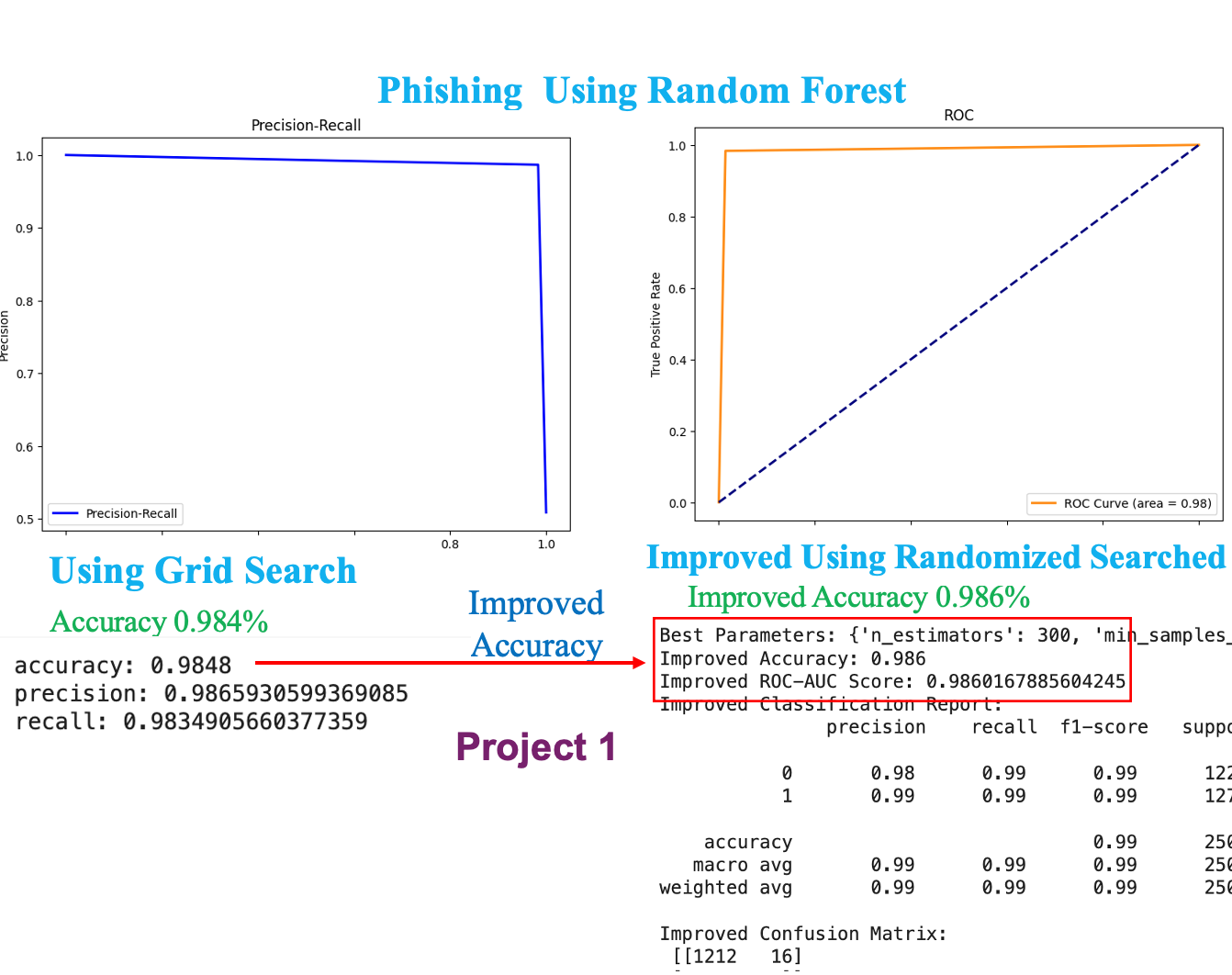
Project 1 Building an AI-driven Phishing detection system is key to cybersecurity. Our journey includes dataset analysis and preprocessing, followed by mastering the logistic regression algorithm.
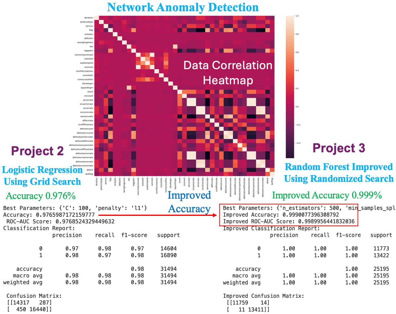
Project 2 The focus is on AI security risks. Our task will be building a network intrusion detection system to detect anomalies and attacks in the network.
• Employ Grid Search or Randomized Search to fine-tune Random Forest hyperparameters, adjusting elements like n_estimators, max_depth, and min_samples_split.
Cross-Validation: • Use GridSearchCV with cross-validation for model consistency across datasets, ensuring robustness and generalizability.
Feature Importance Analysis: • Identify key features influencing the Random Forest model’s decisions to pinpoint network anomaly indicators.
Advanced Model Evaluation: • Deploy confusion matrix, ROC curve, and precision-recall curve for in-depth evaluation. • Calculate metrics like precision, recall, F1-score, and AUC for comprehensive model assessment.
To improve the performance and utilize advanced algorithms for anomaly detection networks, there are several key areas we can focus on:
Algorithm Selection: Logistic Regression is a good start, but we can explore more complex models like Random Forest, Gradient Boosting, or even Neural Networks, which might capture the complexity of the dataset better.
Feature Engineering: Investigating and engineering more relevant features from the existing data can significantly impact the performance.
Model Evaluation: Besides accuracy, we should consider other metrics like Precision, Recall, F1-Score, and ROC-AUC for a more comprehensive evaluation, especially since anomaly detection often deals with imbalanced datasets.
Hyperparameter Tuning: Further tuning of model parameters using techniques like Random Search or Bayesian Optimization.
Data Preprocessing: More advanced techniques in data preprocessing, like handling imbalanced data, feature scaling, and encoding.
import numpy as np
import pandas as pd
import matplotlib.pyplot as plt
from sklearn.ensemble import RandomForestClassifier
from sklearn.metrics import accuracy_score, precision_score, recall_score
from sklearn.model_selection import train_test_split
import matplotlib.pyplot as plt
from sklearn.metrics import roc_curve, auc, precision_recall_curve
from sklearn.metrics import classification_report, confusion_matrix, accuracy_score, roc_auc_score
from sklearn.model_selection import RandomizedSearchCV


# Load dataset
data = pd.read_csv("Phishing_Legitimate_full.csv")

# Data Exploration
data.head()  # Display first five rows
data.info()  # Information about dataset
data.describe()  # Statistical summary
data.max(axis=0)  # Maximum values in each column
data.drop('id', axis=1, inplace=True)  # Drop 'id' column as it's not useful for prediction
data['CLASS_LABEL'].hist()  # Histogram of the class label

# Splitting data into features and labels
X = data.drop("CLASS_LABEL", axis=1)  # Features
y = data["CLASS_LABEL"]  # Labels
X_train, X_test, y_train, y_test = train_test_split(X, y, random_state=42)  # Split data

# Model Training with Random Forest Classifier
model = RandomForestClassifier()
model.fit(X_train, y_train)

# Model Prediction
pred = model.predict(X_test)

# Model Evaluation
accuracy = accuracy_score(y_test, pred)
print("Accuracy:", accuracy)
precision = precision_score(y_test, pred)
print("Precision:", precision)
recall = recall_score(y_test, pred)
print("Recall:", recall)

# ROC Curve
fpr, tpr, _ = roc_curve(y_test, pred)
roc_auc = auc(fpr, tpr)
plt.figure(figsize=(8, 6))
plt.plot(fpr, tpr, color='darkorange', lw=2, label='ROC Curve (area = %0.2f)' % roc_auc)
plt.plot([0, 1], [0, 1], color='navy', lw=2, linestyle='--')
plt.xlabel('False Positive Rate')
plt.ylabel('True Positive Rate')
plt.title('Receiver Operating Characteristic (ROC)')
plt.legend(loc="lower right")
plt.show()

# Precision-Recall Curve
precision, recall, _ = precision_recall_curve(y_test, pred)
plt.figure(figsize=(8, 6))
plt.plot(recall, precision, color='blue', lw=2, label='Precision-Recall')
plt.xlabel('Recall')
plt.ylabel('Precision')
plt.title('Precision-Recall Curve')
plt.legend(loc="lower left")
plt.show()

# Hyperparameter Optimization
param_dist = {
    'n_estimators': [100, 200, 300, 400, 500],
    'max_features': ['sqrt'],
    'max_depth': [10, 20, 30, 40, 50],
    'min_samples_split': [2, 5, 10],
    'min_samples_leaf': [1, 2, 4],
    'bootstrap': [True]
}

# Hyperparameter Tuning using Randomized Search CV
rfs_random = RandomizedSearchCV(estimator=model, param_distributions=param_dist,
                                verbose=1, n_iter=10, cv=5, random_state=42, n_jobs=-1)
rfs_random.fit(X_train, y_train)
print("Best Parameters:", rfs_random.best_params_)

# Best Estimator Evaluation
best_rfs = rfs_random.best_estimator_
rfs_best_pred = best_rfs.predict(X_test)
print("Improved Accuracy:", accuracy_score(y_test, rfs_best_pred))
print("Improved ROC-AUC Score:", roc_auc_score(y_test, rfs_best_pred))
print("Improved Classification Report:\n", classification_report(y_test, rfs_best_pred))
print("Improved Confusion Matrix:\n", confusion_matrix(y_test, rfs_best_pred))
import numpy as np
import pandas as pd
import seaborn as sns
import matplotlib.pyplot as plt
from sklearn.preprocessing import LabelEncoder, MinMaxScaler
from sklearn.model_selection import train_test_split, GridSearchCV
from sklearn.linear_model import LogisticRegression
from sklearn.metrics import classification_report, confusion_matrix, accuracy_score, roc_auc_score

# Load and prepare the dataset
columns = ["duration","protocoltype","service","flag","srcbytes","dstbytes","land",
           "wrongfragment","urgent","hot","numfailedlogins","loggedin", "numcompromised",
           "rootshell","suattempted","numroot","numfilecreations", "numshells","numaccessfiles",
           "numoutboundcmds","ishostlogin", "isguestlogin","count","srvcount","serrorrate",
           "srvserrorrate","rerrorrate","srvrerrorrate","samesrvrate", "diffsrvrate","srvdiffhostrate",
           "dsthostcount","dsthostsrvcount","dsthostsamesrvrate", "dsthostdiffsrvrate",
           "dsthostsamesrcportrate","dsthostsrvdiffhostrate","dsthostserrorrate","dsthostsrvserrorrate",
           "dsthostrerrorrate","dsthostsrvrerrorrate","attack", "lastflag"]

# Loading data
data = pd.read_csv("train.txt", sep=",", names=columns)
data_test = pd.read_csv("test.txt", sep=",", names=columns)

# Data Preprocessing
# Removing irrelevant features
data.drop(['land', 'urgent', 'numfailedlogins', 'numoutboundcmds'], axis=1, inplace=True)

# Handling missing values
data = data.dropna(axis=0)

# Encoding categorical variables
label_encoder = LabelEncoder()
data['protocoltype'] = label_encoder.fit_transform(data['protocoltype'])
data['service'] = label_encoder.fit_transform(data['service'])
data['flag'] = label_encoder.fit_transform(data['flag'])

# Convert 'attack' feature to binary classification
data['attack'] = np.where(data['attack'] != "normal", "attack", "normal")
data['attack'] = label_encoder.fit_transform(data['attack'])

# Data Visualization
# Correlation heatmap
plt.figure(figsize=(20, 15))
sns.heatmap(data.corr())
plt.show()

# Feature Scaling
scaler = MinMaxScaler()
X = data.drop("attack", axis=1)
X = scaler.fit_transform(X)
y = data['attack']

# Splitting data into training and testing sets
X_train, X_test, y_train, y_test = train_test_split(X, y, test_size=0.3, random_state=42)

# Model Training: Logistic Regression
log_reg = LogisticRegression()
log_reg.fit(X_train, y_train)

# Predictions
predictions = log_reg.predict(X_test)

# Model Evaluation
print("Accuracy:", accuracy_score(y_test, predictions))
print("ROC-AUC Score:", roc_auc_score(y_test, predictions))
print("Classification Report:\n", classification_report(y_test, predictions))
print("Confusion Matrix:\n", confusion_matrix(y_test, predictions))

# Hyperparameter Tuning with GridSearchCV
param_grid = {'C': [0.01, 0.1, 1, 10, 100], 'penalty': ['l1', 'l2']}
grid_search = GridSearchCV(log_reg, param_grid, cv=5)
grid_search.fit(X_train, y_train)

# Best Parameters and Improved Predictions
best_params = grid_search.best_params_
print("Best Parameters:", best_params)
improved_predictions = grid_search.predict(X_test)

# Evaluation of Improved Model
print("Improved Accuracy:", accuracy_score(y_test, improved_predictions))
print("Improved ROC-AUC Score:", roc_auc_score(y_test, improved_predictions))
print("Improved Classification Report:\n", classification_report(y_test, improved_predictions))
print("Improved Confusion Matrix:\n", confusion_matrix(y_test, improved_predictions))
Download Train Dataset Download Test Dataset Python Code Download Colab Code Link
import numpy as np
import pandas as pd
import seaborn as sns
import matplotlib.pyplot as plt
from sklearn.ensemble import RandomForestClassifier
from sklearn.metrics import classification_report, confusion_matrix, accuracy_score, roc_auc_score
from sklearn.model_selection import RandomizedSearchCV
from sklearn.preprocessing import MinMaxScaler
from sklearn.preprocessing import LabelEncoder
from sklearn.model_selection import train_test_split

# Define column names for the dataset
columns = ["duration","protocoltype","service","flag","srcbytes","dstbytes","land", "wrongfragment","urgent","hot","numfailedlogins","loggedin", "numcompromised","rootshell","suattempted","numroot","numfilecreations", "numshells","numaccessfiles","numoutboundcmds","ishostlogin",
"isguestlogin","count","srvcount","serrorrate", "srvserrorrate",
"rerrorrate","srvrerrorrate","samesrvrate", "diffsrvrate", "srvdiffhostrate","dsthostcount","dsthostsrvcount","dsthostsamesrvrate", "dsthostdiffsrvrate","dsthostsamesrcportrate",
"dsthostsrvdiffhostrate","dsthostserrorrate","dsthostsrvserrorrate",
"dsthostrerrorrate","dsthostsrvrerrorrate","attack", "lastflag"]

"""
#Downlod link for dataset directly
https://www.kaggle.com/datasets/anushonkar/network-anamoly-detection
"""

# Data Preprocessing
# Dropping irrelevant features
data = pd.read_csv("Train.txt", sep= ",", names=columns)
data_test = pd.read_csv("Test.txt", sep= ",", names=columns)
data.shape
data.head()
data.describe()
data.info()
data.drop(['land', 'urgent', 'numfailedlogins', 'numoutboundcmds'],axis=1, inplace=True)

#Preprocessing to data_test
data_test.drop(['land', 'urgent', 'numfailedlogins', 'numoutboundcmds'], axis=1, inplace=True)
data_test.fillna(0, inplace=True)  # Assuming you want to fill missing values with 0
data.shape
data.isna().sum()

# Handling missing values in the training dataset
clean_data = data.dropna(axis=0)
clean_data.select_dtypes(exclude=[np.number])
clean_data.shape
data['attack'].unique()
data ['attack'] = np.where(data['attack'] != "normal", "attack", "normal")
data ['attack'].unique()

#Remove object type from dataset
le = LabelEncoder()
data [ 'protocoltype'] = le.fit_transform(data['protocoltype'])
data [ 'service'] = le.fit_transform(data['service'])
data [ 'flag'] = le.fit_transform(data['flag'])
data [ 'attack'] = le.fit_transform(data['attack'])
data.info()

# Feature correlation visualization
plt.figure(figsize=(20, 15))
sns.heatmap(data.corr())

#Sorting data
scaler = MinMaxScaler()
clean_data = data.dropna(axis=0)
X = clean_data.drop("attack", axis=1)
y = clean_data['attack']
X.fillna(0, inplace=True)

# Feature Scaling
scaler = MinMaxScaler()
X_scaled = scaler.fit_transform(X)

# Splitting the dataset
X_train, X_test, y_train, y_test = train_test_split(X_scaled, y, test_size=0.2, random_state=42)
X_train.shape
X_test.shape

# Random Forest Model Training with Hyperparameter Tuning
param_dist = {
    'n_estimators': [100, 200, 300, 400, 500],
    'max_features': ['sqrt'],
    'max_depth': [10, 20, 30, 40, 50],
    'min_samples_split': [2, 5, 10],
    'min_samples_leaf': [1, 2, 4],
    'bootstrap': [True]
}

# Using RandomForest
rf = RandomForestClassifier()

# Hyperparameter tuning using RandomizedSearchCV
rf_random = RandomizedSearchCV(estimator=rf, param_distributions=param_dist, verbose=1, n_iter=10, cv=5, random_state=42, n_jobs=-1)
rf_random.fit(X_train, y_train,verbose=1)

# Displaying the best parameters
print("Best Parameters:", rf_random.best_params_)

# Model Evaluation with the best estimator
best_rf = rf_random.best_estimator_
rf_best_pred = best_rf.predict(X_test)

# Evaluation Metrics
print("Improved Accuracy:", accuracy_score(y_test, rf_best_pred))
print("Improved ROC-AUC Score:", roc_auc_score(y_test, rf_best_pred))
print("Improved Classification Report:\n", classification_report(y_test, rf_best_pred))
print("Improved Confusion Matrix:\n", confusion_matrix(y_test, rf_best_pred))
Download Train Dataset Download Test Dataset Python Code Download Colab Code Link
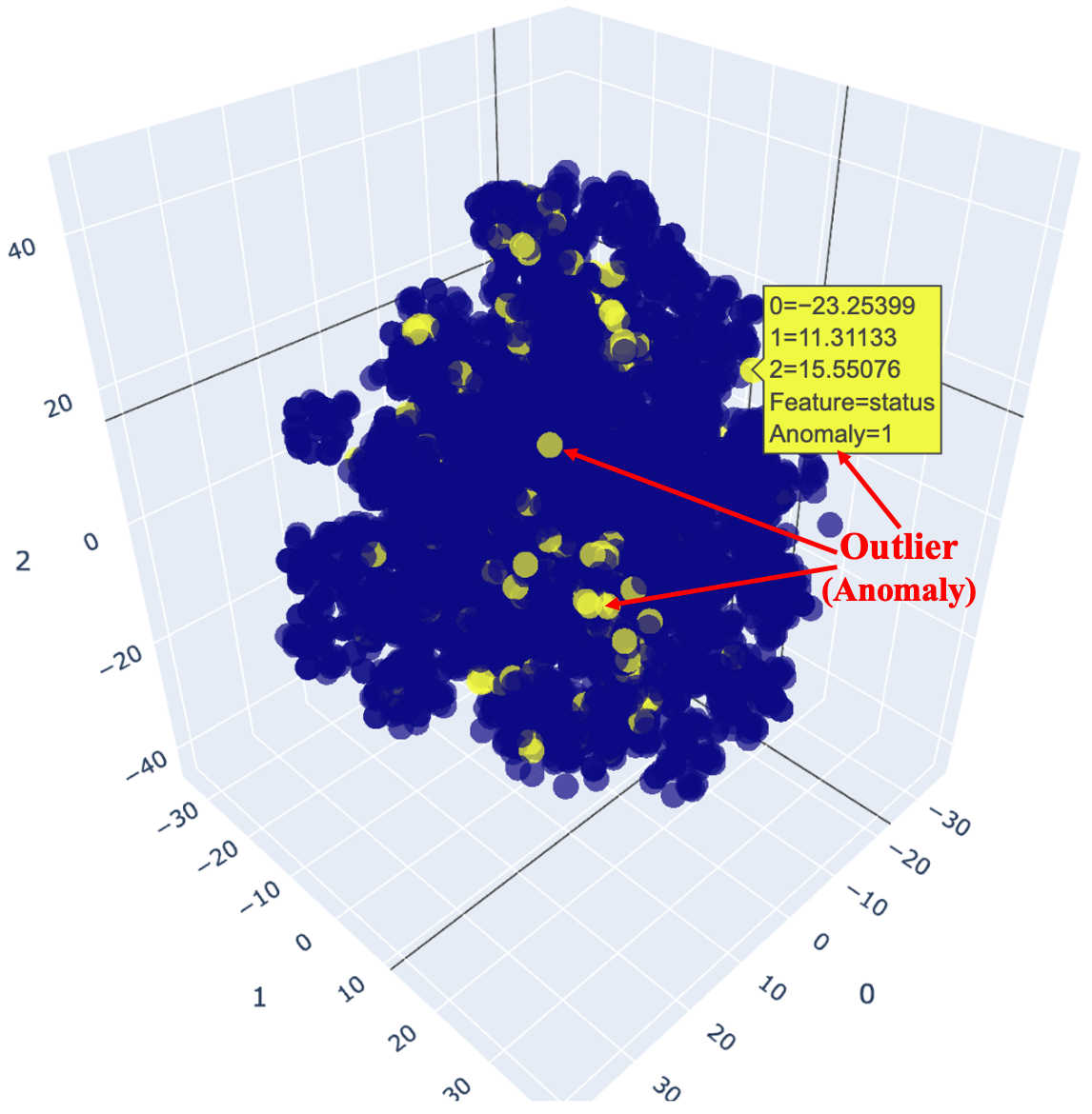
Anomalies, or outliers, are points of data that deviate from the standard pattern. They can indicate potential risks needing attention or opportunities to capitalize on, such as an unexpected increase in sales of a product. Anomaly Detection Algorithm Summary:b
Isolation Forest
• Mechanism: Isolation Forest identifies outliers by randomly selecting features and partitioning data, isolating anomalies effectively.
• Strengths: Quick and scalable, handles extensive feature sets well, and is less influenced by outlier quantity.
• Weaknesses: Less effective for correlated feature datasets, as it treats each feature in isolation.
Local Outlier Factor (LOF)
• Mechanism: LOF calculates local density deviations to pinpoint outliers, identifying points with significantly lower density compared to neighbors.
• Strengths: Proficient with high-dimensional data and complex feature relationships.
• Weaknesses: Intensive computation for large datasets, parameter selection is critical.
K-Nearest Neighbors (KNN)
• Mechanism: KNN detects outliers by assessing the distance to an instance's k-nearest neighbors, flagging significant distance disparities.
• Strengths: Straightforward and versatile, accommodates various data types and feature scales.
• Weaknesses: Sensitive to the choice of 'k' and can be computationally heavy for large datasets.
In conclusion, the choice of outlier detection algorithm will depend on the characteristics of the data and the specific requirements of the task. Isolation Forest and LOF are suitable for high-dimensional data, while KNN is simple and effective for different types of data. Experimental evaluation algorithms on the data help to choose the one that best meets the requirements of the task.
• Library Installation and Importing:
Installs PyCaret.
Imports necessary libraries including PyCaret for anomaly detection, Pandas for data manipulation, Plotly for visualization, and Google Colab for file operations.
• Data Loading:
Reads an IoT dataset from a CSV file, iot_data.csv.
Parses dates in the 'timestamp' column.
• Data Preprocessing:
Removes an unnamed column which likely doesn't contain relevant information.
Sets 'timestamp' as the index of the DataFrame and converts it to a DateTime object for time series analysis.
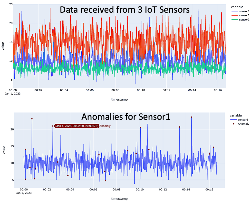
• Data Visualization:
Visualizes the entire dataset using a line plot to understand trends or patterns.
• Setup for Anomaly Detection with PyCaret:
Initializes the PyCaret environment with the dataset.
Lists available models in PyCaret for anomaly detection.
• Anomaly Detection Model Creation:
Creates an Isolation Forest (iforest) model, setting the fraction of outliers (anomalies) in the data.
Assigns the model to the dataset, effectively labeling data points as normal or anomalous.
• Filtering Out Anomalies:
Extracts the anomalous results from the dataset for further analysis or action.
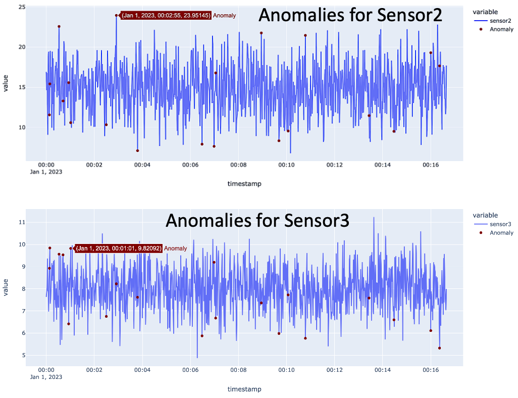
• Anomaly Visualization:
Plots sensor data (e.g., 'sensor1') over time.
Highlights anomalies on the plot using maroon markers, providing a visual representation of where anomalies occur in the time series.
!pip install pycaret
"""# Libararies"""

from pycaret.anomaly import *
from google.colab import files
import io
import pandas as pd
import plotly.graph_objects as go
import plotly.express as px

"""#Load data"""

df = pd.read_csv(('iot_data.csv'), parse_dates=['timestamp'])
print(df.head())

"""# Remove column without info and update dataset"""

df = df.drop(columns=['Unnamed: 0'])

df.set_index('timestamp', inplace=True)

df.index = pd.to_datetime(df.index)

"""#Visualize data"""

fig = px.line(df)
fig.show()

"""#See Structure of Dataset"""

s = setup(df, session_id = 123)

# list of available models in pyCaret
models()

"""# Detection"""

#Create model, choosing fractional value  is depending on the feasibility and importance of responding to IOT alerts
ifo = create_model('iforest', fraction = 0.02)
iforest = assign_model(ifo)

"""## Filter out anomolies"""

#filter out anomalous results
anomalousresults = iforest[iforest['Anomaly'] == 1]

anomalousresults.shape

"""#Plot Results"""

# Plot result of selected sensor "sensor1" on y-axis, date information on x-axis
plt = px.line(iforest, x=iforest.index, y=["sensor1"], title='IOT Data ANOMALY DETECTION')

#identify anomolies(outliers) in plot
anomaly = iforest[iforest['Anomaly'] == 1].index

# Plots detection of Sensor1  data
y_values = [iforest.loc[i]['sensor1'] for i in anomaly]
plt.add_trace(go.Scatter(x=anomaly, y=y_values, mode = 'markers', name = 'Anomaly', marker=dict(color='maroon',size=6)))
plt.show()